Build your own layers for deep learning models using TensorFlow 2.0 and Python

Jun 23, 2020 8 min read

Project

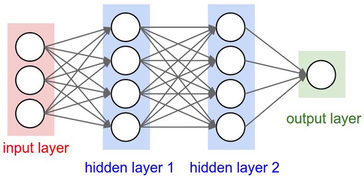Image : Stack Overflow

Background

During a very recent webinar where I was a speaker for the topic Deep learning with TensorFlow I repeatedly was asked a question regarding how would one really define their own layers, parameter and how they work so as to watch it do the magic while showing them some notebooks that had parameters to the layers that we regularly use. This prompted me to write a blog explaining layers and their parameters.

Building Tensorflow Layers

The tf.keras.layers.Layer or also written as tf.compat.v1.keras.layers.Layer gives you easy and effective access to start writing your own layers in building the desired convolutional neural network. Keras backend is well integrated with TensorFlow giving you ease of coding your layers at a high level understanding and handles a ot of code that you would otherwise would’ve written.

Writing your own layers is not that daunting if you have a certain understanding on how they work. According to the TensorFlow documentation

Many machine learning models are expressible as the composition and stacking of relatively simple layers, and TensorFlow provides both a set of many common layers as a well as easy ways for you to write your own application-specific layers either from scratch or as the composition of existing layers.

Which is pretty much True in the sense that these layers can be written like calling functions with arguments. Here in the tf.keras.layers package the layers that we want to define are treated as objects. So to construct a simple layer by yourself all you need is to construct the layer object and you are pretty much good to go.

Some widely used layers include

Conv1D
Conv2D
AvgPool1D
Dense
Flatten
LSTMCell

and many more. To start defining your own layers is no hidden secret and can be easily achieved by doing (we will be looking at Sequential layers here)

model = tf.keras.models.Sequntial()

or


model = tf.compat.v1.keras.Sequential()

or


model = tf.compat.v1.keras.models.Sequential()

Here the most important task of defining the type of your layers is done. Let’s look at some of these layers and their functions one by one. Once you are ready with your network or at least have an idea of how many layers you would like to write for a standard result you can proceed to now defining them. What Sequential essentially does it groups a linear stack of layers. Once you have done that now you are ready to construct your own layer objects.

After declaring above you can either do

model = tf.keras.models.Sequential()

model.add(tf.keras.layers.Dense(8, input_dim=16))

model = tf.keras.Sequentail([ tf.keras.layers.Dense(8, input_dim=18)])

Both these methods will help you achieve your goal of writing your own layers. To begin with let’s build our own complete network and understand each parameters.

model = tf.keras.models.Sequential([
  
  tf.keras.layers.Conv2D(64, (3,3), activation='relu', input_shape=(28, 28, 1)),

  # Max pooling as we will take maximum value which is a 2X2 poll so every 4 pixels go to 1
  tf.keras.layers.MaxPooling2D(2, 2),

  # Another layer
  tf.keras.layers.Conv2D(64, (3,3), activation='relu'),
  tf.keras.layers.MaxPooling2D(2,2),

  # Converts the input to 1D set instead of the square we saw earlier
  tf.keras.layers.Flatten(),

  # Adds a layer of neurons
  tf.keras.layers.Dense(128, activation='relu'),

  # The last layers have specific number of neurons, ask me why! :)

  tf.keras.layers.Dense(10, activation='softmax')
])

Now once we have built our layer, let’s try to understand it one by one. We have already seen in brief about Sequential(), let’s now dive into the layers. The module tf.keras.layers.Layer has different classes defined for all different kinds of models some of which are also listed above.

In the first layer Conv2D(64, (3,3), activation='relu', input_shape=(28, 28, 1)), refers to class Conv2D.
- This layers creates a conv kernel to convolve with input to produce tensors.
- Activation function needs to be defined here and also if this layer is being used as the first layer in this model as shown in this example it is important to include input_shape as in input_shape = (128, 128, 3) for an image that is 128 X 128 pixel wide with three channels mainly RGB or use 1if it is a grey scale image.
- Arguments here include :
  - the filter size as 64 , which creates 64 filters to convolve over the input.
  - the size of the kernel which is defined as (3, 3).
  - activation is set to as relu, what ReLU activation in brief means that the output values from this activation function are positives as all values in the left of the number line are counted as 0.
  - the input_shape as defined above here is an grey scale image with size 28 X 28 pixels hence (28, 28, 1). Input shape can be defined as (batch_size, rows, cols, channels) to understand order and meaning of the parameters.
  - other arguments which can be added are strides, padding, use_bias and many more based on the requirements.
The second layer tf.keras.layers.MaxPooling2D(2, 2), is a maxpooling layer for which more information can be found here.
- This layers creates a max pooling operation for 2D spatial data.
- Arguments here include :
  - MaxPooling is used to down-sample the data or the input to it by taking the maximum value from the window defined by pool_size which here is (2, 2).
  - The window is shifted by strides which are values by which we define by how many pixels our window moves ahead through the input representations.
  - If padding is defined as same the output shape becomes output shape = input_shape / strides and output shape = (input_shape - pool_size + 1) / strides) when padding size is defined as valid.
  - This returns 4D tensor representing maximum pooled values.
The third layer tf.keras.layers.Flatten() which is a layer in between the convolutional layer and a fully connected layer.
- As evident from the name it flattens the input into a 1D vector that can be fed to a fully connected classifier layer.
- The main argument here data_format as when inputs are shaped (batch,) without a channel dimension, then flattening adds an extra channel dimension and output shapes are (batch, 1) - TFDocs. In this case the input is 28X28X3 with 64 filter which makes the output of the Flatten layer to 64X28X28 = 50176 as a 1D vector instead of multi-dimension as in previous layers.
The fourth layer tf.keras.layers.Dense(10, activation='softmax') adds a single layer to your network which is densely or fully connected.
- Each neuron declared here is connected to or receives input from all neurons from previous layers hence the name as densely connected.
- Dense implements the operation: output = activation(dot(input, kernel) + bias) where activation is the element-wise activation function passed as the activation argument, kernel is a weights matrix created by the layer, and bias is a bias vector created by the layer (only applicable if use_bias is True). - TFDocs
- The final layer is the layer that can be described here as output layer. The number 10 here is the number of classes that we are fed or the number of outputs that are to be observed.
- One needs to understand that the output is not however a one shot yes or no but a list of probabilities of all the classes wherein then the highest probability is the prediction done by the model.
- More importantly we are using the function softmax here which in simple words mean that the highest probability will be treated as 1 and all others as 0. This might sound somewhat like maxpool but these are two different concepts. Softmax function can also be loosely defined as the function that converts logits to probabilities that sum to 1. In short if the result of classes is like [0.1, 0.4, 0.5] then the Softmax will return [0, 0, 1] . Known use-cases of softmax regression are in discriminative models such as Cross-Entropy and Noise Contrastive Estimation.

Writing your own layers becomes more important when you want to build a fully custom solution which otherwise cannot be achieved using transfer learning(although being an decent method if you want a prototype). This helps you understand the tool you are using here TensorFlow and also get an understanding of how SoTA neural netwrks work and what do those layers mean or how the authors reached to those specific parameter values. We have networks ranging from 20 layers to more than a 100 with huge complexity which we aim to ease here by understanding the design process.

I would also suggest going through the Tensorflow documentation extensively as they are a offiial resource of class and functions available in the TensorFlow API with a very good description of every parameter in detail.

In a jiffy

We took a look at a higher level understanding of various TensorFlow layers, what do they mean and what do their arguments mean in brief. You can start building your own model from scratch(well let’s say just calling classes and functions :) ) and test them out by tuning various parameters mentioned and from the function definitions too and maybe you’ll soon have a best performing model in your profile. Happy coding!

Code for reference | GitHub | Website |

References :

[1] Tensorflow documentation - https://www.tensorflow.org/api_docs/python/tf

[2] Softmax function simpplified - https://towardsdatascience.com/softmax-function-simplified-714068bf8156

[3] Wikipedia

[4] Coursera - Tensorflow lectures by Laurence Moroney